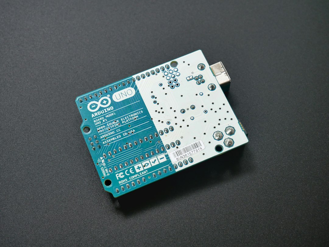
The Challenge of Non-Linearity in Embedded Systems
In the world of Arduino-based engineering, the jump from "hobbyist project" to "precision instrument" is almost always defined by the quality of data acquisition. While many tutorials introduce the map() function—a linear interpolation tool—real-world sensors rarely behave linearly. Whether you are working with thermistors, pressure transducers, or specialized gas sensors, their physical response often follows an exponential, logarithmic, or power-law curve.
When you attempt to force-fit a linear model onto a non-linear signal, you inevitably introduce systematic error. This error manifests as "dead zones" at the ends of your sensor's range or significant drift in the middle. Polynomial curve fitting for non-linear sensor calibration acts as the mathematical bridge, allowing your microcontroller to translate raw ADC (Analog-to-Digital Converter) counts into high-fidelity physical units.
The Mathematical Foundation of Polynomial Regression
Polynomial curve fitting involves finding the best-fitting curve for a set of data points by minimizing the sum of the squares of the vertical deviations. In the context of an Arduino project, you are essentially solving for the coefficients of a polynomial equation:
$y = a_n x^n + a_{n-1} x^{n-1} + ... + a_1 x + a_0$
Where:
- $y$ is the physical output (e.g., temperature in Celsius, pressure in kPa).
- $x$ is the raw ADC input value (0–1023 or 0–4095).
- $a_n$ are the coefficients derived during the calibration phase.
For most sensors, a second-order (quadratic) or third-order (cubic) polynomial provides an excellent balance between computational simplicity and high accuracy. Higher-order polynomials are rarely needed and often lead to "overfitting," where the model maps to the noise of your calibration set rather than the actual physical trend.
Data Acquisition: The Calibration Workflow
Before writing a single line of code, you must build a robust dataset. A poor calibration dataset will result in a poor model, regardless of how elegant your algorithm is.
- Define Your Range: Identify the minimum and maximum expected values for your application.
- Establish Ground Truth: Use a high-precision reference instrument (a calibrated thermometer, a digital pressure gauge) to measure the physical property simultaneously with your sensor.
- Data Collection: Capture at least 10–20 data points across the entire operating range. Do not cluster them; space them out to capture the curvature of the sensor’s response.
- Regression Analysis: Use external software (like Excel, Google Sheets, or Python/NumPy) to plot your $(x, y)$ data points and generate a "Trendline." Ensure you select "Display Equation on Chart."
Implementation in Arduino C++
Once you have your coefficients from your regression software, implementing them in your Arduino sketch is straightforward. You must be mindful of the float data type to maintain precision during calculation.
Best Practices for Algorithm Optimization
When implementing the equation, avoid calculating powers using the pow() function, as it is computationally expensive on 8-bit AVR microcontrollers. Instead, use simple multiplication:
```cpp
// Instead of: y = apow(x, 2) + bx + c;
// Use:
float x = analogRead(A0);
float y = (a x x) + (b * x) + c;
```
This optimization significantly reduces clock cycles, allowing for higher sampling rates in control loops.
Comparison: Linear vs. Polynomial vs. Look-up Tables
Choosing the right calibration strategy depends on the memory and processing constraints of your specific hardware.
| Strategy | Accuracy | Memory Footprint | Computational Load | Ease of Setup |
|---|---|---|---|---|
| Linear Map | Low | Ultra-Low | Negligible | Very Easy |
| Polynomial Fit | High | Low | Moderate | Moderate |
| Look-up Table | Very High | High | Low | Complex |
| Spline Interpolation | Very High | Moderate | High | Difficult |
As shown in the table, polynomial curve fitting offers the best "bang for your buck" regarding memory usage versus accuracy, making it ideal for the Arduino Uno, Nano, and ESP32 platforms.
Signal Filters and Noise Mitigation
Polynomial fitting assumes the raw input $x$ is accurate. However, electrical noise is the enemy of calibration. If your ADC value is jittering, your polynomial calculation will produce "noisy" results even if the model is perfect.
Moving Average Filters
Before passing the ADC value into your polynomial equation, implement a simple moving average filter. This buffers the last N readings and returns the average. This effectively smooths out high-frequency transients without needing complex DSP (Digital Signal Processing) libraries.
Kalman Filtering
For mission-critical applications where sensor movement is dynamic (e.g., drone altitude or automotive speed sensing), a Kalman filter is superior to a simple moving average. It dynamically adjusts its weight based on the uncertainty of the measurement, providing a stable, fast-reacting input for your calibration polynomial.
Testing and Validation
Never skip the validation phase. After hardcoding your coefficients into the Arduino sketch, perform a "blind test." Measure a set of values that were not used to generate the original polynomial coefficients. If the calculated output matches the reference instrument within your acceptable error margin, your calibration is successful. If the error is too high, evaluate whether a higher-order polynomial (e.g., cubic) is required or if you need to perform "piecewise calibration"—splitting the sensor's range into two separate polynomials for different operating segments.